You can deploy OpenFold3-preview from Amazon SageMaker JumpStart. The OpenFold Consortium and the AlQuraishi Lab at Columbia University developed OpenFold3 as an open source biomolecular structure prediction model. With a few lines of code, you can typically deploy OpenFold3 into your own AWS account. You can then predict the 3D structures of proteins, DNA, RNA, small-molecule ligands, and the complexes they form. The endpoint runs with network isolation, which you can use to help keep your sequences within your AWS account.
Computational drug discovery teams now use structure prediction as a core part of their work. Teams use it in target identification, antibody and protein engineering, and structure-based virtual screening. Teams have found running these models challenging. You need GPU infrastructure, a working CUDA and PyTorch stack, large model checkpoints, and a serving layer that handles requests that take minutes rather than milliseconds. SageMaker JumpStart can handle much of that work for you. OpenFold3 runs in an AWS-maintained container on a managed Amazon SageMaker AI endpoint. The endpoint is designed to handle request queuing and GPU warmup, and you can add autoscaling.
In this post, we show you how to:
- Deploy OpenFold3-preview on a SageMaker asynchronous inference endpoint.
- Submit structure prediction jobs and interpret the results, including predicted structures and confidence scores.
- Run several predictions in parallel on multi-GPU instances.
- Supply your own multiple sequence alignments (MSAs) to improve prediction accuracy while helping keep your sequences private.
- Help reduce costs by scaling your endpoint to zero when it’s idle.
Overview of OpenFold3
OpenFold3 is an all-atom structure prediction model. It predicts the joint 3D structure of a set of molecules from their sequences. It isn’t limited to single protein chains: It can fold multi-chain protein complexes, protein–nucleic acid assemblies, and protein–ligand complexes in one prediction.
| Attribute | Details |
| Developer | OpenFold Consortium / AlQuraishi Lab, Columbia University |
| Model type | All-atom biomolecular structure prediction |
| Inputs | Protein, DNA, and RNA sequences. Small-molecule ligands as SMILES |
| Outputs | Predicted structures in mmCIF format, with confidence metrics (pLDDT, PAE, PDE) |
| Version | OpenFold3 0.4.1, of3-p2-155k checkpoint |
| License | Apache 2.0 |
| JumpStart model ID | huggingface-proteinfolding-openfold3 |
| Supported instances | ml.g6.2xlarge, ml.g6.4xlarge (default), ml.g6.12xlarge |
The OpenFold3 developers release its code and model weights under the Apache 2.0 license, and they publish the training data and methods. Research organizations and pharmaceutical companies can inspect the model, fine-tune it, and build on it under the terms of that license. The developers describe OpenFold3-preview as a research preview.
Use cases
- Target and complex structure prediction – Predict structures for targets that have no experimental structure, including multi-chain assemblies and protein–nucleic acid complexes.
- Protein–ligand co-folding – Fold a protein together with a small molecule supplied as SMILES to generate binding-pose hypotheses for structure-based design.
- Antibody and protein engineering – Evaluate designed variants by predicting their structures and comparing confidence across candidates.
- High-throughput screening pipelines – Queue large batches of prediction jobs against an autoscaling endpoint and process the results directly from Amazon Simple Storage Service (Amazon S3).
Why OpenFold3 uses asynchronous inference
Most JumpStart models, such as large language models and embedding models, deploy to real-time endpoints. A real-time endpoint returns its response within a single request, and that request is capped at 60 seconds. Structure prediction works differently. Folding time grows with the number and length of the chains in a query, and real-world proteins and complexes often take several minutes.
For this reason, OpenFold3 on JumpStart runs on SageMaker Asynchronous Inference:
- You upload the request to Amazon S3 and call
InvokeEndpointAsync, which returns immediately. - The endpoint queues the request and processes it, with an invocation timeout of up to 1 hour.
- The endpoint writes the result, or the error details, to an S3 location you choose. You can poll for it or get a notification through Amazon Simple Notification Service (Amazon SNS).
Two properties of asynchronous endpoints suit scientific workloads especially well. First, they queue bursts of requests internally, so you can submit a large batch of sequences without building your own job queue. Second, they can scale to zero instances when the queue is empty, which helps you avoid paying for idle instances between experiments.
Prerequisites
To follow this walkthrough, you need:
- An AWS account, and a SageMaker AI execution role for the endpoint. Following least privilege, this AWS Identity and Access Management (IAM) role needs read and write access only to the S3 prefix that you use for requests and results. For more information, see How to use SageMaker AI execution roles.
- IAM permissions for the identity that runs the code: to create, describe, invoke, and delete the model, endpoint configuration, and endpoint, plus
iam:PassRolefor the execution role. For the optional scale-to-zero section, it also needs AWS Application Auto Scaling and Amazon CloudWatch alarm permissions. In production, scope these permissions to your resources rather than using broad managed policies such asAmazonSageMakerFullAccess. For more information, see Complete the prerequisites for asynchronous inference. - Access to Amazon SageMaker Studio, a SageMaker notebook instance, or a local IDE.
- The SageMaker Python SDK v3 and py3Dmol, which you can install with
pip install "sagemaker>=3,<4" py3Dmol. - Service quota for at least one
ml.g6.4xlargeendpoint instance in your AWS Region. You also need quota forml.g6.12xlargeif you follow the multi-GPU section. You can check your quotas and request increases in the Service Quotas console under Amazon SageMaker.
Important: SageMaker endpoints are billed per instance-hour while they’re running, including while they’re idle. To avoid unexpected charges, follow the Clean up section, or configure scale-to-zero as described later in this post. For pricing details, see Amazon SageMaker AI pricing.
Discover OpenFold3 in SageMaker JumpStart
- Open SageMaker Studio and choose JumpStart in the navigation pane.
- Search for OpenFold3.
- Open the model card to review the model description, license, and supported instance types.
- Open the example notebook from the model card. It contains the complete asynchronous deployment walkthrough shown in this post.
Deploy OpenFold3 with the SageMaker Python SDK
First, build the model from its JumpStart configuration and define an AsyncInferenceConfig. The output and failure paths are the S3 locations where the endpoint writes results and error details.
import json, time, uuid
import boto3
from sagemaker.core.helper.session_helper import Session
from sagemaker.core.inference_config import AsyncInferenceConfig
from sagemaker.core.jumpstart.configs import JumpStartConfig
from sagemaker.core.training.configs import Compute
from sagemaker.serve.model_builder import ModelBuilder

session = Session()
bucket = session.default_bucket()          # sagemaker-{region}-{account-id}
prefix = "openfold3-async"

model_builder = ModelBuilder.from_jumpstart_config(
    jumpstart_config=JumpStartConfig(
        model_id="huggingface-proteinfolding-openfold3",
        accept_eula=True,
    ),
    compute=Compute(instance_type="ml.g6.4xlarge"),
)
model = model_builder.build()

async_config = AsyncInferenceConfig(
    output_path=f"s3://{bucket}/{prefix}/output",
    failure_path=f"s3://{bucket}/{prefix}/failure",
)

endpoint = model_builder.deploy(inference_config=async_config)
endpoint_name = endpoint.endpoint_name
print(f"Deployed asynchronous endpoint: {endpoint_name}")
Setting accept_eula=True confirms that you’ve reviewed and accepted the model’s license terms, which is required to deploy this model. If you run this code outside SageMaker Studio, also pass your SageMaker execution role to ModelBuilder.from_jumpstart_config with role_arn="<role-arn>".
The endpoint stores your requests and results in Amazon S3, and they contain your sequences and predicted structures. For proprietary sequences, consider using a dedicated S3 bucket or prefix with server-side encryption using an AWS Key Management Service (AWS KMS) key that you manage. To encrypt results with your key, pass its ARN to AsyncInferenceConfig as kms_key_id. Restrict access with a bucket policy that allows only the roles that run this workflow, and add an S3 Lifecycle rule to expire request and result objects that you don’t need to keep. For more information, see Security best practices for Amazon S3.
Deployment typically completes within minutes. This includes a warmup step in which the container runs a short prediction on each GPU, so that the GPUs are warmed up when the endpoint reaches InService.
Tip: G6 capacity can be limited in some Regions. If a deployment fails with
InsufficientInstanceCapacity, retry later, choose a different supported instance size, or deploy in another AWS Region where the model is available.
Run a structure prediction
A request is a JSON document with one or more named queries, and each query lists its chains. All chains in a query are folded together as one complex. Separate queries are folded independently.
Each chain has these fields:
molecule_type–protein,dna,rna, orligand.chain_ids– a list of chain identifiers, such as["A"]. To specify identical copies, such as a homodimer, use["A", "B"].sequence– the residue sequence, for protein, DNA, and RNA chains.smiles– a SMILES string, used for ligand chains instead ofsequence.
The following example folds human ubiquitin, a well-characterized 76-residue protein:
s3 = boto3.client("s3")
smr = boto3.client("sagemaker-runtime")

payload = {
    "queries": {
        "ubiquitin": {
            "chains": [
                {
                    "molecule_type": "protein",
                    "chain_ids": ["A"],
                    "sequence": "MQIFVKTLTGKTITLEVEPSDTIENVKAKIQDKEGIPPDQQRLIFAGKQLEDGRTLSDYNIQKESTLHLVLRLRGG",
                }
            ]
        }
    }
}

# 1. Stage the request in S3
input_key = f"{prefix}/input/{uuid.uuid4().hex}.json"
s3.put_object(Bucket=bucket, Key=input_key, Body=json.dumps(payload).encode())

# 2. Submit asynchronously -- returns immediately
resp = smr.invoke_endpoint_async(
    EndpointName=endpoint_name,
    ContentType="application/json",
    InputLocation=f"s3://{bucket}/{input_key}",
    InvocationTimeoutSeconds=3600,
)
output_location, failure_location = resp["OutputLocation"], resp["FailureLocation"]
Then poll S3 for either the result or a failure record:
def split(uri):
    b, _, k = uri.removeprefix("s3://").partition("/")
    return b, k

result = None
for _ in range(120):                                    # up to ~30 minutes
    for loc, is_failure in ((output_location, False), (failure_location, True)):
        try:
            body = s3.get_object(Bucket=split(loc)[0], Key=split(loc)[1])["Body"].read()
        except s3.exceptions.NoSuchKey:
            continue
        if is_failure:
            raise RuntimeError(body.decode())
        result = json.loads(body)
    if result:
        break
    time.sleep(15)

if result is None:
    raise TimeoutError(f"No result yet; check {output_location}")
if result.get("status") == "error":
    raise RuntimeError(result["error"])
A request with invalid input, such as a malformed chain or an unsupported MSA name, still produces a result object, but with "status": "error" and an error message instead of structures. The last check surfaces that message.
Prediction time grows with the size of the input. In our tests on ml.g6.4xlarge, smaller proteins completed more quickly than larger proteins.
Interpret the results
The response contains a status, a list of predicted structures in mmCIF format, and their matching confidences. By default, OpenFold3 generates five diffusion samples per query, so each query returns five candidate structures. Each sample comes with two confidence files: a detailed one (*_confidences.json) and a summary (*_confidences_aggregated.json). The summary includes a sample_ranking_score that you can use to pick the best sample.
import os
os.makedirs("structures", exist_ok=True)
for s in result["structures"]:
    path = os.path.join("structures", os.path.basename(s["filename"]))
    with open(path, "w") as f:
        f.write(s["content"])
    print("saved", path, f'({s["size_bytes"]/1024:.0f} KB)')

summaries = {c["filename"]: c["data"] for c in result["confidences"]
             if c["filename"].endswith("_aggregated.json")}
for name, m in sorted(summaries.items(), key=lambda kv: -kv[1]["sample_ranking_score"]):
    print(f'{name}: ranking={m["sample_ranking_score"]:.2f} pLDDT={m["avg_plddt"]:.1f} '
          f'pTM={m["ptm"]:.2f} ipTM={m["iptm"]:.2f}')
You can open the .cif files in any structure viewer, such as PyMOL, ChimeraX, or Mol*. To view a structure inline in a notebook, use py3Dmol:
import py3Dmol   # pip install py3Dmol
view = py3Dmol.view(width=600, height=450)
view.addModel(result["structures"][0]["content"], "cif")
# pLDDT is stored in the B-factor field: red = low confidence, blue = high
view.setStyle({"cartoon": {"colorscheme": {"prop": "b", "gradient": "roygb", "min": 50, "max": 90}}})
view.zoomTo(); view.show()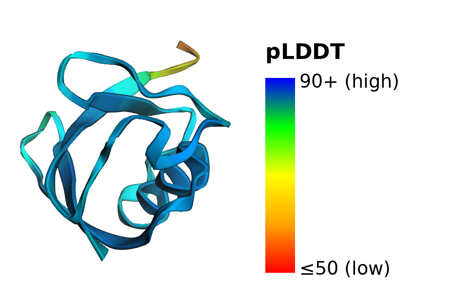
Figure 1: OpenFold3’s predicted structure of ubiquitin, rendered with the preceding code and colored by per-atom confidence (pLDDT). All figures in this post were rendered with 3Dmol.js (Rego and Koes, Bioinformatics, 2015).
The prediction shows ubiquitin’s compact fold: a mixed beta-sheet packed against a single alpha-helix. Most of the structure is blue (high confidence). Only the flexible C-terminal tail, at the top of the image, shifts toward yellow and red, which matches the tail’s known flexibility in experimental structures.
The confidence metrics tell you how much to trust each prediction:
- pLDDT (predicted local distance difference test) – Per-atom confidence in the local structure, on a scale of 0–100. Higher is better, and values above about 70 generally indicate a reliable local structure. The summary file reports the average as
avg_plddt. - pTM and ipTM (predicted TM-score and interface pTM) – Overall confidence in the fold, and in how chains and ligands are positioned relative to each other, on a scale of 0–1. For complexes, ipTM is the key number. The summary file also reports
chain_pair_iptmfor each pair of chains. - PAE (predicted aligned error) and PDE (predicted distance error) – Per-residue-pair error estimates, in the detailed confidence file. Use them to judge the relative placement of domains and chains.
Fold a complex
To predict a complex, list several chains in the same query. The following example co-folds human carbonic anhydrase II with its catalytic zinc ion and the drug acetazolamide. This is a well-studied complex with experimental structures in the Protein Data Bank (for example, PDB 3HS4):