This article explains how LLMs encode and process token position information by covering classic and contemporary methods like RoPE. It’s essentially a comprehensive journey where we will work through the mechanisms with visual examples, a little math, and a small PyTorch implementation. And, of course, we will then also look at how modern architectures adapt or omit explicit positional encodings.
Below, you can find a preview of which positional embedding choices are used in 2026 open-weight models. We will discuss these choices later after covering the underlying mechanisms.
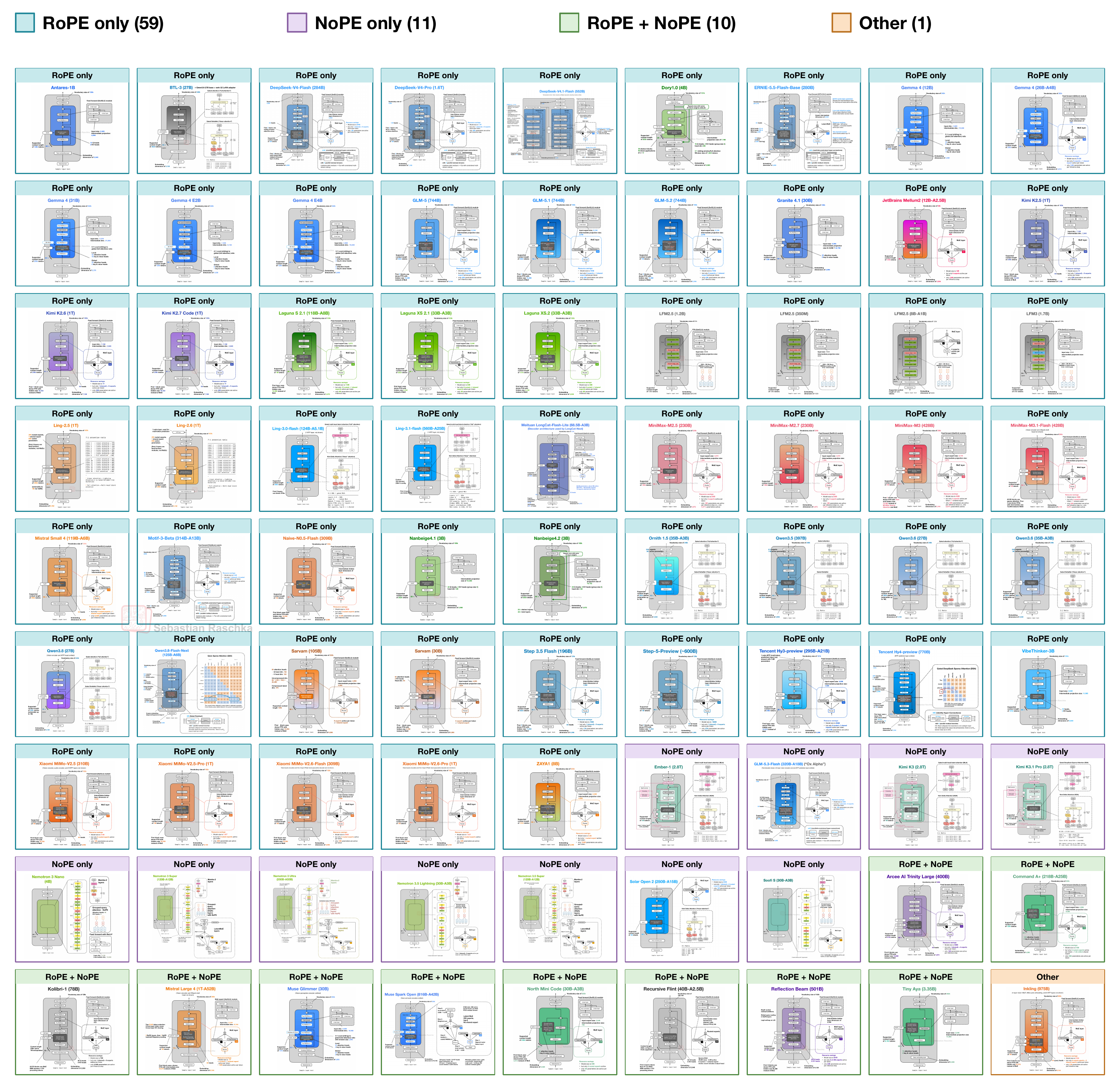
But why spending so much time writing/reading about this rather minor building block? LLMs keep evolving, and as I was preparing a new article on the latest LLM architecture trends this year, I realized that I never covered the positional information methods used in LLMs in any article so far. So, instead of letting the other article get out of hand, I thought it might make sense to publish this as a standalone building block for the upcoming LLM architecture and trends analysis.
Also, over the years, many readers have asked me for a tutorial on relative positional embeddings (aka RoPE) to follow up on the learned absolute embeddings used in GPT. It’s been on my TODO list for a long time, so I finally revisited my old draft and put this walkthrough together, which will cover
different positional methods in LLMs;
(finally) how RoPE works;
what methods are used by recent open LLMs.
Note that this article assumes some familiarity with basic LLM architectures and works well as a follow-up to Build a Large Language Model (From Scratch). If the concepts and computation of the attention internals, particularly query, key, and value vectors, are a little fuzzy, I recommend checking my self-attention walkthrough as a refresher:
The article is also very technical and likely too detailed for some. However, I really wanted to have this foundation out there for future articles to reference. And no worries, the next one will return to a more comfortable style.
PS: I started experimenting with Substack’s new “perks” system. As a thank-you to supporters, I’ve added image exports and metadata from the architecture gallery for you to use in your own analyses.
PPS: If you are already familiar with how position embeddings work, feel free to fast-forward to Section 6, Positional choices in modern architectures.
Note that this article may be best read in a web browser than an email client. I recommend checking out the web view here, which also has a navigation bar on the left side.
1. Where position information enters an LLM
Let’s start with the overall architecture. A tokenizer encodes the input text into token IDs. Next, the input token embedding layer of an LLM maps each of these IDs to a vector of numbers. We usually refer to these entries in that vector as “features” (similar to classic ML). The transformer blocks inside the LLM then modify these vectors using attention and feedforward layers. Lastly, the model’s output layer produces logit scores (converted into probabilities) for the next token.
The following shows this path in GPT-2 (a relatively classic LLM) and MiniMax-M3 (a more recent LLM released this year; a placeholder for most other recent LLMs). As we can see, the architectures are not too different from each other, but before we get to the positional information parts, let’s focus on the orange blocks for now (the token embedding layers) and the transformer blocks above them; the other architecture differences aren’t needed for this explanation.
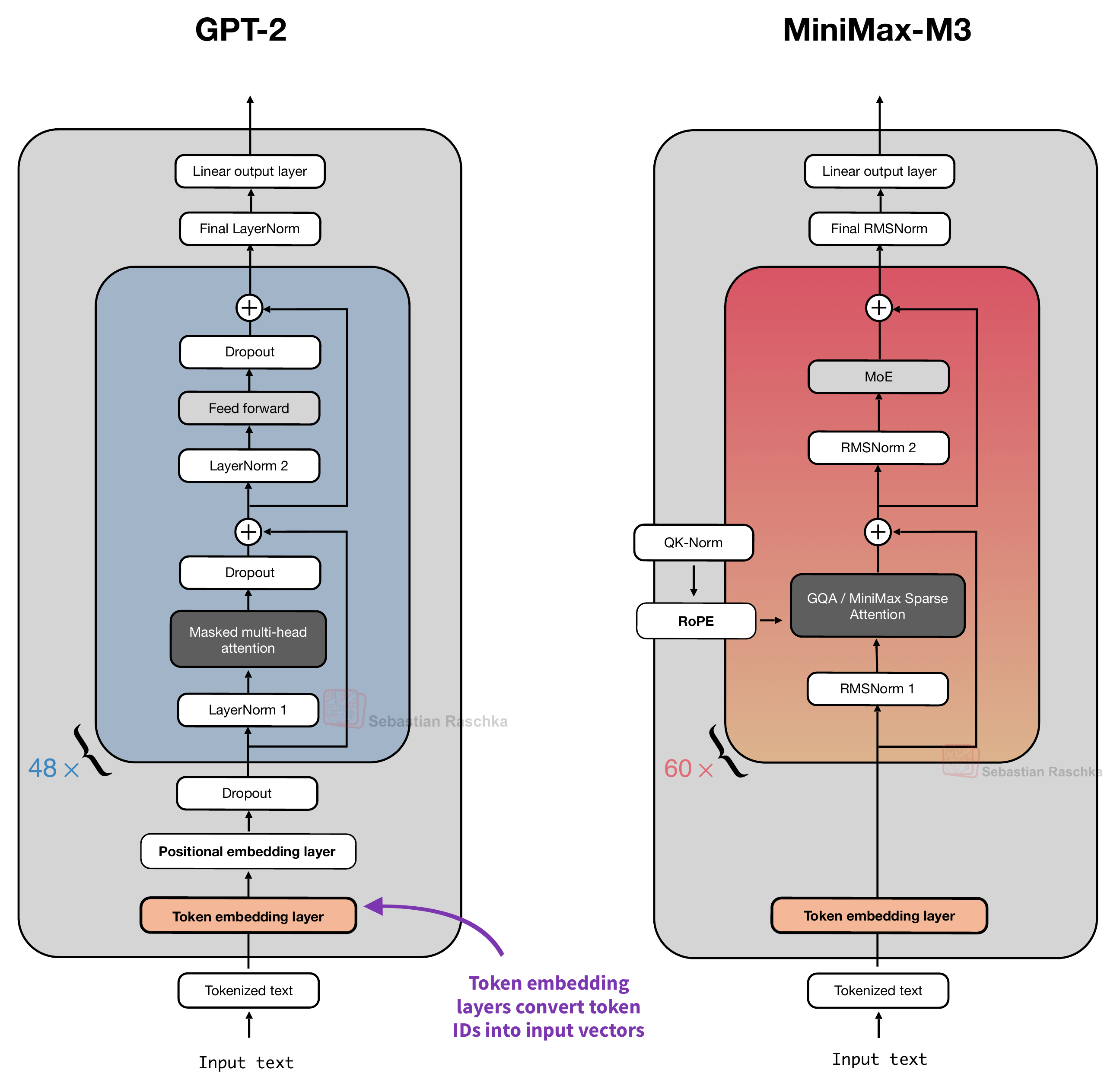
A token embedding layer, shown in the figure above, maps each token ID to a vector. Position information is then added afterward. Concretely, and as we will discuss in more detail later, GPT-2 adds a position vector to each token embedding before the modified embedding enters the first transformer block. On the other hand, MiniMax-M3 adds the positional information in each transformer block using a method called RoPE inside attention.
We will talk about these methods in more detail later, but first, let’s start with the big picture information explaining why explicit positional information is added or needed.
1.1 Why add positional information?
Consider the following two input sentences as a simple example:
“The red fox jumps over the gray fox.”
“The gray fox jumps over the red fox.”
Changing the word order changes which fox does the jumping, as illustrated in the following figure.
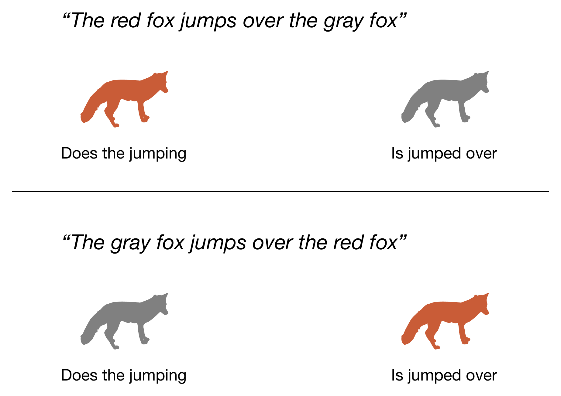
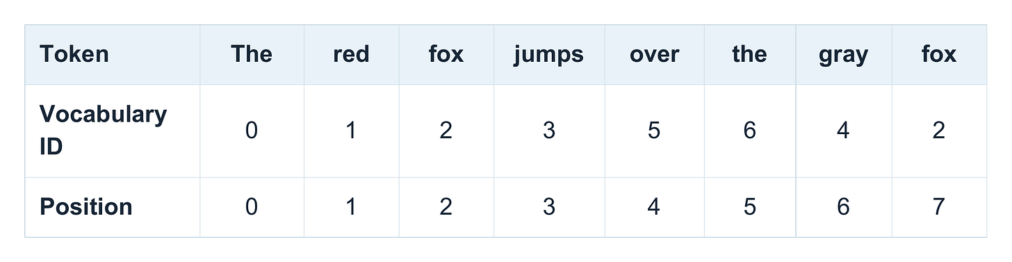
For the examples in this article, we will treat each word as one token for simplicity. (As you know, real tokenizers can split words into smaller subword tokens.) The first sentence then has eight token positions, from 0 through 7.
# Assume the following small vocabulary.
# Real vocabularies typically have 50k to 200k entries
vocab = {
    "The": 0,
    "red": 1,
    "fox": 2,
    "jumps": 3,
    "gray": 4,
    "over": 5,
    "the": 6,
}
(If you are interested in how vocabularies are built, check out my tokenizer materials on GitHub.)
Note that “fox”, which appears twice in the input sentence, gets the same token ID 2 in both cases. And since they both have the same token ID, irrespective of the position in the input sentence, they would get the same embedding vector from the embedding layer.
Now, let’s consider a regular self-attention mechanism with no positional encoding (and no causal mask), where every input token can attend to every other token in the input. In this scenario, swapping any two words, like “red” and “gray”, would still result in the same embeddings and attention scores between each token pair.
GPT-style models do use a causal (autoregressive) mask, which restricts each token to itself and earlier tokens. Interestingly, this causal mask gives the computation some implicit order information. In our example, “jumps” can attend to “red” in the first sentence and “gray” in the second. So, a causal LLM can theoretically already distinguish these sentences even without explicit positional embeddings. (We will return to this idea later when discussing the “NoPE” concept.)
Nonetheless, GPT-2 and most newer LLMs include explicit positional information because it gives attention a direct signal about positions. That’s because even though the causal mask determines which tokens are accessible and provides implicit order information, it doesn’t distinguish a separation of one position from a separation of ten, for example. So, explicit positional methods are still useful (or even essential), since they supply that information.
If this all sounded confusing, don’t worry, it was more meant as an overview, and we will step through these concepts a bit more slowly in the remaining article.
2. Adding a position vector to each token embedding
We briefly talked about implicit positional information through causal attention masks (and we will revisit this again in more detail later). However, we now switch gears and talk about the explicit ways to add positional information.
The perhaps simplest and most direct (but not “cheapest”) approach is to give each sequence position its own vector. We add that vector to the token embedding, so the resulting, modified embedding vector is then passed to the first transformer block. This exact procedure is discussed in the following subsections.
2.1 Learned absolute position embeddings in GPT-2
To illustrate the use of an explicit, learned positional vector to the input embeddings, let’s consider GPT-2 as a concrete example. GPT-2 learns a table of position vectors during training. The following figure illustrates where these vectors are used in the architecture, that is, immediately after the token embedding lookup and before the first transformer block.
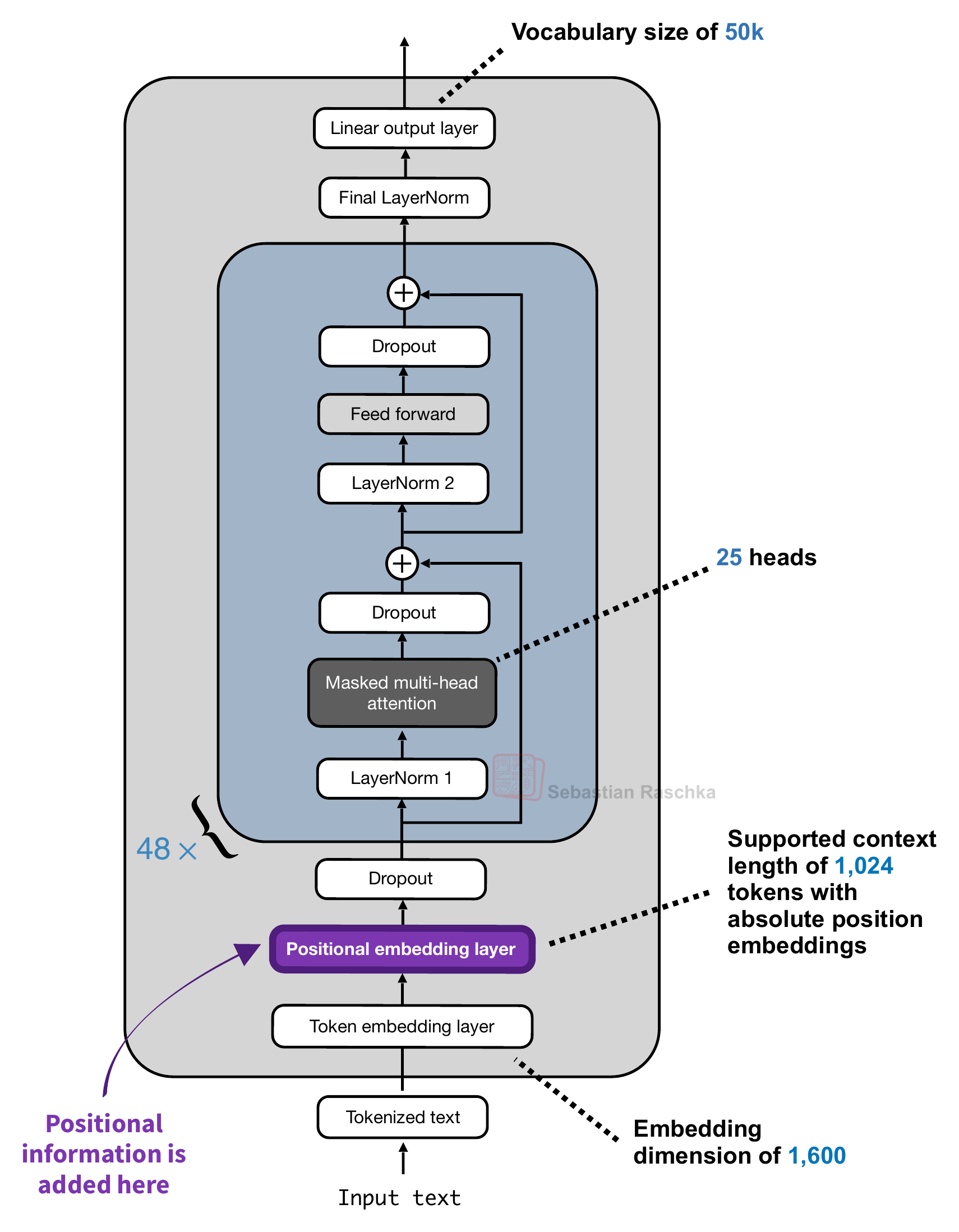
The positional embedding layer depicted in the figure above follows the same implementation as the token embedding layer, i.e., they have exactly the same output dimensions so that the resulting input vectors can be added to each other. The code below shows that with an excerpt of a GPT-2 code implementation:
class GPTModel(nn.Module):
    def __init__(self, cfg):
        super().__init__()
        self.tok_emb = nn.Embedding(cfg["vocab_size"], cfg["emb_dim"])
        self.pos_emb = nn.Embedding(cfg["context_length"], cfg["emb_dim"])
        self.drop_emb = nn.Dropout(cfg["drop_rate"])

        self.trf_blocks = nn.Sequential(
            *[TransformerBlock(cfg) for _ in range(cfg["n_layers"])])

        self.final_norm = LayerNorm(cfg["emb_dim"])
        self.out_head = nn.Linear(
            cfg["emb_dim"], cfg["vocab_size"], bias=False
        )

    def forward(self, in_idx):
        batch_size, seq_len = in_idx.shape
        tok_embeds = self.tok_emb(in_idx)
        pos_embeds = self.pos_emb(torch.arange(seq_len, device=in_idx.device))
        x = tok_embeds + pos_embeds  # Shape [batch_size, num_tokens, emb_size]
        x = self.drop_emb(x)
        x = self.trf_blocks(x)
        x = self.final_norm(x)
        logits = self.out_head(x)
        return logits
And in mathematical terms, we can write it as follows. Let m be a position index and xm the token ID at that position. The input to the first block is

Here,
Etoken is the embedding layer,
Pm is the position info vector selected by m,
and hm is the resulting summed embedding and position vector.
The two vectors have the same width, so we add their entries element-wise. Figure 6 below shows this visually with a small numerical example.
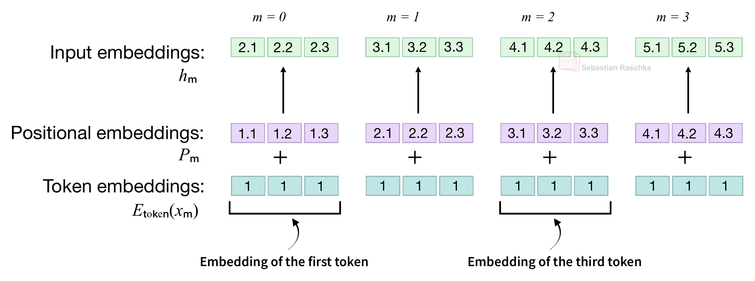
In the figure above, at position 0, adding the token embedding [1, 1, 1] to the position embedding [1.1, 1.2, 1.3] gives [2.1, 2.2, 2.3]. By the way, the values in the figure are chosen to keep the illustration simple; in a real example, both embedding layers (tables) are initialized with small random values and learned during training.
So, what we covered in this section is a so-called absolute positional method because the positional embedding Pm depends on the token’s own position m. In the previous example sentence, the two “fox” tokens have initially the same token embeddings, but because we are adding different positional vectors P2 and P7, they have different values before they enter the first transformer block. And consequently, the query, key, and value vectors inside the attention mechanisms then also receive representations that already include position information.
Note that the original GPT-2 implementation has 1,024 learned position vectors. This means it only works with inputs with 1024 or fewer tokens. If we want to extend the context window, we would have to extend this embedding table. And since the embedding table (layer) is updated like any other layer during training, the context length would have to be decided before the training starts.
Extending the context would be very expensive since the table can become very large. For example, in the case of GPT-2 Medium, the positional embedding layer weights only make up 0.30% of the total weights at 1,024 positions. However, if we increased the context length to a nowadays common 100k range, they would make up >22% of the total model weights, which would be very uneconomic.
2.2 Fixed sinusoidal position encodings in the original transformer
The original “Attention Is All You Need” transformer from 2017, which predates GPT, uses the same addition mechanism, but computes its position vectors with fixed sine and cosine functions. Figure 7 below shows this addition before both the encoder and decoder stacks. The encoder processes the input sequence, and the decoder generates the output sequence. (The reason why it’s introduced here is that th